With an explosion of scientific interest in graphene based material for its incredible electronic, optical, and physical properties; it became clear that we needed to develop a cost effective instrument that could be used for quality determination as well as characterization. Raman spectroscopy has long been the most versatile tool for this; however, with Graphene’s low Raman scatter, frequent impurities, and low laser damage thresholds typically only high-end Raman microscopy systems (costing hundreds of thousands of dollars) were available for the job. Here we present a new lower cost instrument, the StellarNet HYPER-Nova, which bridges this performance gap. Also, we discuss some of the more practical issues surrounding Raman spectroscopy of Graphene as well as many useful features for graphene characterization found in its Raman spectrum.
Introduction
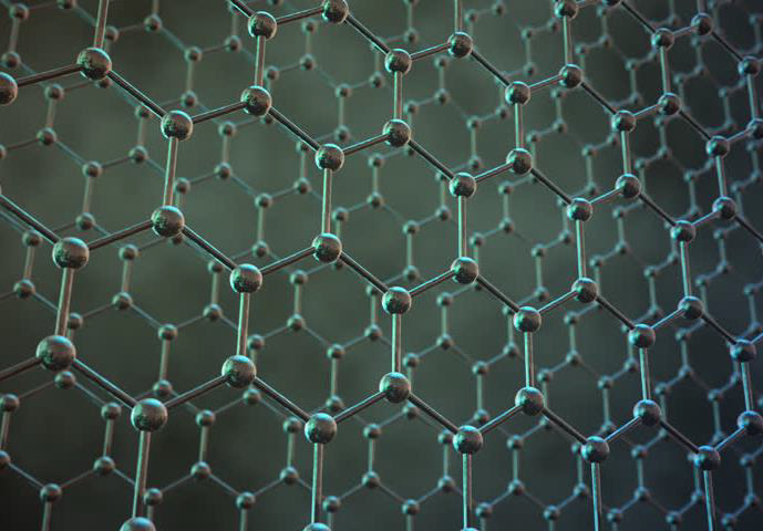
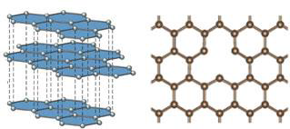
Graphene is truly the material of the future. Discovered in 2004 by Professor Sir Andre Geim and Professor Sir Kostya Novoselov of the University of Manchester, Graphene displays many unique electronic, optical, and physical properties. Graphene is an allotrope of carbon consisting of a single layer of carbon atoms arranged in a hexagonal lattice.
It is a semi-metal with very high electrical conductivity (near-ballistic transport) with high specific surface area and high thermal conductivity which makes it a promising material for high-frequency nanoelectronics, micro-mechanical systems, thin-film transistors,
batteries, and supercapacitors with ultra-high charging speeds. Graphene’s unique optical properties produce an unexpectedly high opacity for an atomic monolayer and can be seen with the naked eye. This allows for potential uses in flexible optoelectronics or even used as smart wallpaper collecting unused photons and recycling them throughout your house! Graphene is amazingly tough and lightweight. It is the strongest material ever discovered having more than 300 times the tensile strength of structural steel and Kevlar! Its hexagonal shape provides a great barrier for larger molecules which leads to uses in membrane and filtration chemistry, gas sensing, rust resistance and durable material coatings.
The peak in scientific interest over the past several decades has sparked developments in the preparation methods for Graphene and related materials as well as the need for cost-effective scientific instrumentation for characterization and quality determination.
Some techniques such as micromechanical exfoliation, chemical vapor deposition, and epitaxial growth on silicon carbide typically produce higher quality monolayer Graphene while other artificial fabrication routes such as the reduction of a Graphene Oxide (GO) solution and organic synthesis, tend to introduce defects into the Graphene. Typical defects might include vacancies and dislocations, as well as exposing the graphene to oxidation, hydrogenation, fluorination, and other chemical functionalizations. Graphene can also be decomposed into one-dimensional and zero-dimensional forms, such as graphene nanoribbons and nanographene.
The Raman Spectrum of Graphene
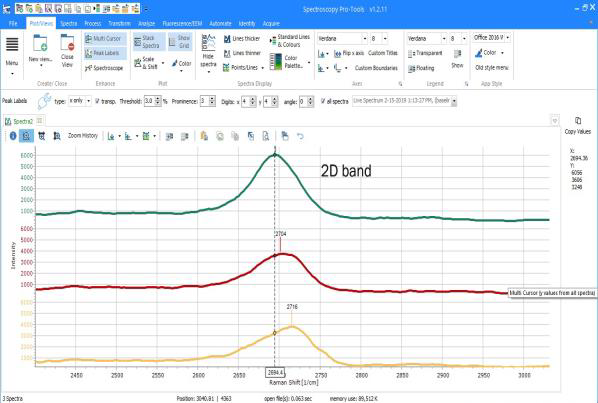
The Raman spectrum of Graphene and related materials is fairly simple, consisting of just a few typical bands. Analyzing the position and shape of these Raman bands can tell us quite a lot about the carbon material’s properties. Below, you can see a typical Graphene sample showing D, G, and the 2D bands.
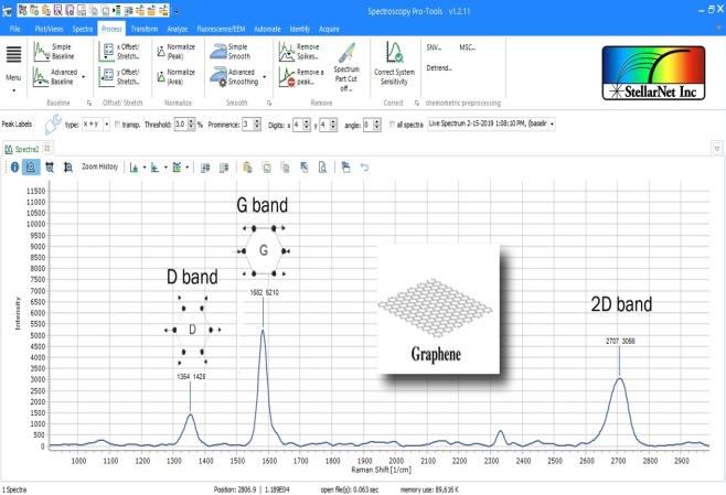
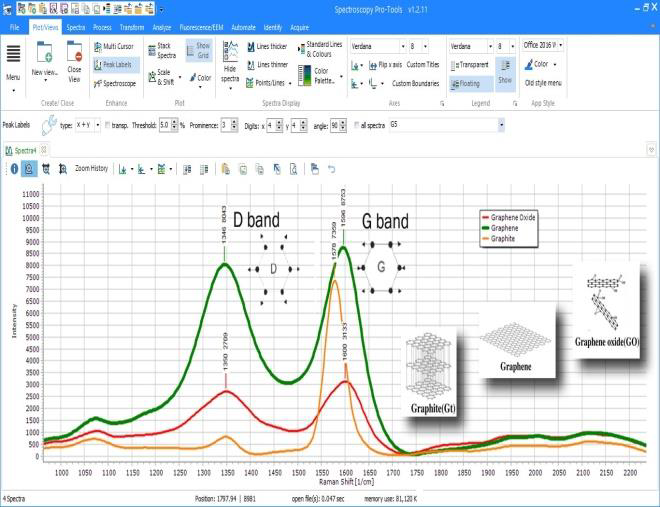
The Raman spectra of Graphite and a Graphene Oxide are very similar as we would expect since graphite is composed of multilayer Graphene. The three main bands in the Graphene spectrum are known as the D-band at ~1350 cm-1, the G-band at ~1582 cm-1 and the 2D band at ~2685 cm-1. In Graphite the D band is usually very weak and G band is much sharper. A comparison of Graphene, Graphite, and Graphene Oxide Raman spectra can be seen below as well as their molecular structures.
The G-band
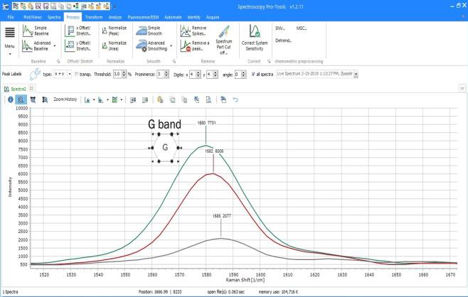
The G-band is the primary mode in Graphene related materials. It represents the planar configuration of sp2 bonded carbons. The band position is independent of excitation laser frequency, making it different from the other Graphene bands. The position of the band and its shape can provide useful information for material characterization. One common application for G-band analysis in Graphene is for layer thickness determination. Figure 3 demonstrates the effect that layer thickness has on the position of the G-band. As the layer thickness increases the band position shifts. This shift to lower energy represents a slight softening of the bonds as layers increase. The measured positions of the bands in Figure 3 are representative of the calculated positions. It should be noted that the position of the G-band is quite sensitive to doping and even very minor strain. This needs to be considered when attempting to use the position of this band to determine Graphene layer thickness.
The D-band
The D-band is also considered the ‘disorder’ band or the ‘defect’ band and is not present in pristine samples. One generally refers to defects in Graphene as anything that breaks the symmetry of the infinite carbon honeycomb shaped lattice. The D-band represents a ring breathing mode from sp2 carbon rings. To be active the ring must be adjacent to a Graphene edge or a defect.
The band is the result of a single phonon lattice vibrational process. The band is typically very weak in Graphite and is typically weak in high quality Graphene as well. A significant peak in the D-band indicates that there are many defects in the material. The intensity, peak position, and line width of the Raman modes can significantly change with the increasing number of defects. Another important note on the D-band is that it is a resonant band. This means that it exhibits what is known as dispersive behavior. Because of this the choice of excitation laser is important when analyzing and comparing the spectra due to the number of very weak modes underlying this band.
The 2D-band
The 2D-band is the second order of the D-band. Sometimes this band is referred to as an overtone of the D-band. Unlike the D-band, it does not need to be adjacent to a defect to be active. It is the result of a two phonon lattice vibrational process. Because of this, the 2D-band is always a strong band in Graphene and is present even when there is no D-band present. This band does not represent defects. Like the G-band, the 2D-Band is also used when trying to determine Graphene layer thickness. However, the differences between single and multilayer Graphene in this band are more complex than a simple band shift.
Note that while there is a general shifting to higher wavenumbers as the layer thickness increases, the more noticeable changes have to do with the band shape. The changes in band shape have to do with changes to the active components of the vibration. With single layer Graphene, there is only one component to the 2D-band, but with multilayer Graphene, there are several components to the 2D-band. This is why the shape of the band is so different.
Finally, it is also worth noting that the 2D-band is very sensitive to Graphene folding, which needs to be considered when trying to use this band to determine layer thickness in samples.
Practical Measurement Considerations
When choosing a Raman instrument for Graphene characterization there are a few factors to consider. Here we discuss some of them from an application standpoint.
Cost-effectiveness of Instrumentation
First and foremost, many of the current market solutions for Graphene analysis are expensive high-end Raman microscopy systems, precluding most from easy characterization. In many cases, both academic and industrial departments/research groups share a single machine which is booked between many users. Here, we present a lower cost modular system for Graphene analysis using a laser module, Raman probe, and our HYPER-Nova deep cooled and back thinned Raman spectrometer, with options for microscopy.
Laser Frequency and Power
Graphene is commonly deposited on Si or SiO2 substrates. It is important to consider this aspect of your Graphene measurement as these
materials can exhibit high fluorescence with NIR lasers (such as 785nm). While it is possible to do Graphene characterization with many different excitation wavelengths, visible lasers such as 633nm or 532nm are typically recommended.
Laser power is also very important for Graphene analysis. Exciting your sample with too much laser power will cause your sample to burn. StellarNet’s standard Laboratory Lasers come with power adjustment knobs to decrease or increase laser light to your samples. In some cases, such as 532nm excitation, a fiber optic attenuator is used to manually decrease green light to your sample to prevent burning.
Using a Microscope
Although it is not necessary, using a microscope such as the StellarSCOPE saves time and frustration. Optimizing laser power and adjusting focus can be accomplished in just a few minutes. To optimize laser power first start with a low power and gradually increase until part of your sample burns. You can use the microscope to visually verify that you have ignited your sample. Next, reduce the power and re-adjust the position for your next measurement.
Likewise, in order to optimize your focus spot you can view your sample and use the microscope’s position adjustment knobs until your Graphene comes into focus.
Again, the microscope is not 100% necessary but reduces time spent measuring nothing at all or unfocused locations on your sample.
Sample Preparation
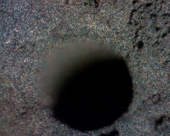
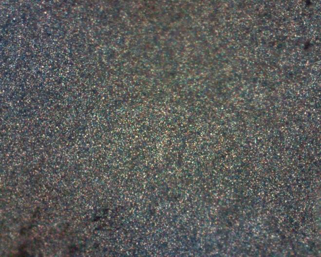
Another important factor in characterizing Graphene is in the preparation. Often the carbon material can present itself as light and fluffy and have an extremely uneven surface. It is important that the sample be compacted or pelletized to have the most even surface possible. Due to the fact that the Raman scatter is fairly weak and requires long detector exposure times it is important not to use any slides or vials that may have impurities in them which will create their own signals.
Choice of Detector
The StellarNet new HYPER-Nova spectrometer uses a research grade back-thinned CCD that is deep cooled to -60 degrees C and has RMS noise values ~20 counts at 3 minutes, which compares to our typical Raman-HR-TEC with ~500 RMS counts at the same exposures. This new instrument achieves the best Signal to Noise of any StellarNet spectrometer and really has been designed out of necessity to bridge the performance gap between high-end instrumentation and our off-the-shelf Raman spectrometers.
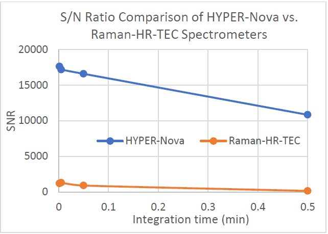
The HYPER-Nova can meet the performance requirements necessary to capture low Raman scatter from Graphene while maintaining resolution to monitor band shifts and shape changes. This new type of high performance modular system will make Graphene characterization more widely available to researchers and help further increase scientific interest in graphene based materials.
If you have further questions about Raman spectroscopy feel free to contact Kaplan Scientific for more information. info@kaplanscientific.nl